2 model setup

2.1 Aim: Read in environmental data and physiology functions

3 File information

~/Library/CloudStorage/Box-Box/Sarah and Molly’s Box/FHL data/code/set_up_workspace/Model_20210409_iter_small_barnacles_food.2.R

This is now set up to work with the desktop computer (different working directory) -1/20/21

This sets up all of the data and functions for the model predictions

This model is calibrated with Lisa’s data, and includes padilla bay chlorophyll seasonal data. To go back to Lisa’s dataset and check the calibration, please use this model setup.

This model uses lengths rather than tissue mass samples. Go back to previous models, e.g. Model_202006.._iter… for tissue mass

4 Datasets used are within the following directories:

If the file is opened within the .Rproj file, then the function here::here() will find the correct data file regardless of where this is being run. An alternative option is to set the root drive using knitr, but I’m having trouble doing this with quarto. Quarto seems to require that all the .qmd files live within the root directory.

5 Set up environment

Clear the global environment

rm(list = ls())

Load libraries and set graphics theme:

Loading required package: stats4

Loading required package: Matrix

Loading required package: carData

lattice theme set by effectsTheme()
See ?effectsTheme for details.


Attaching package: 'nlme'

The following object is masked from 'package:lme4':

    lmList

Loading required package: viridisLite

Loading required package: timechange


Attaching package: 'lubridate'

The following objects are masked from 'package:base':

    date, intersect, setdiff, union


Attaching package: 'dplyr'

The following object is masked from 'package:nlme':

    collapse

The following object is masked from 'package:bbmle':

    slice

The following objects are masked from 'package:stats':

    filter, lag

The following objects are masked from 'package:base':

    intersect, setdiff, setequal, union


Attaching package: 'tidyr'

The following objects are masked from 'package:Matrix':

    expand, pack, unpack


Attaching package: 'zoo'

The following objects are masked from 'package:base':

    as.Date, as.Date.numeric


Attaching package: 'gridExtra'

The following object is masked from 'package:dplyr':

    combine


Attaching package: 'kableExtra'

The following object is masked from 'package:dplyr':

    group_rows

Toggle the period of interest (which 6 month period - the first or second?)

#Time period 1 or 2
timing <- 1

Toggle the subset of barnacles used (specify only small baracles will be used for calculations)

#Which subset of barnacles
small_only<-"Y"

Toggle plots on and off (turning plotting off will speed up the code)

#Turn plotting on and off (for the sake of speeding up the iterations)
figs <- "Y" #(Y or N)

More toggles

#Food dynamics hypothesis
PadillaBay = "Y"

#Test run?
baby_model <- "Y" #Test run
baby_model <- "N" #All data

Set up dataframes to be used in plotting functional responses

#| echo: false

# Plotting values for functional responses

pred.dat <- data.frame(
  Temp.n = rep(seq(from = 5, to = 40, length.out = 20), times = 3),
  OperculumLength = rep(c(4.5, 5.5, 6.5),times = 3,each = 20),
  sizeclass = as.factor(rep(c("small","medium", "large"),times = 3,each = 20))
)

pred.dat.aqua <- data.frame(
  Temp.n = rep(seq(from = 5, to = 20, length.out = 20), times = 3),
  OperculumLength = rep(c(4.5, 5.5, 6.5),times = 3,each = 20),
  sizeclass = as.factor(rep(c("small","medium", "large"),times = 3,each = 20))
)

pred.dat.air <- data.frame(
  Temp.n = rep(seq(from = 5, to = 40, length.out = 20), times = 3),
  OperculumLength = rep(c(4.5, 5.5, 6.5),times = 3,each = 20),
  sizeclass = as.factor(rep(c("small","medium", "large"),times = 3,each = 20))
)

Set up climate change calculator

6 Read in opercular length growth data

Previous directories included: setwd(“C:/Users/eroberts/Box/PhotoAnalysis_Sp2020/datasheets_org/20201007_data”) setwd(“~/Box/PhotoAnalysis_Sp2020/datasheets_org/20201007_data”) setwd(“~/Box/PhotoAnalysis_Sp2020/FHL/datasheets_org/20201007_data”)

and setwd(“~/Box/Sarah and Molly’s Box/FHL data/growth_individual/ForSam_20201007”)

and setwd(“~/Library/CloudStorage/Box-Box/PhotoAnalysis_Sp2020/FHL/datasheets_org/20201007_data/probably final data set”)

# Note the here() function finds the file from the root directory. The root directory is set from running through the project in github. 
growth.1 <- read.csv(here::here("data/growth_data/Scaled_data_Feb_Aug.csv"))
growth.2 <- read.csv(here::here("data/growth_data/Scaled_data_Aug_Mar.csv"))

# Quality control
growth.2 <- growth.2[growth.2$Elevation!="",] #one line of NA's
growth.1 <- growth.1[growth.1$growth.Aug.Feb>=-.1,] #one line of an outlier with a growth of >-0.1

# Structure dataframe
growth.1$Elevation <- as.factor(growth.1$Elevation)
growth.2$Elevation <- as.factor(growth.2$Elevation)

# Subset by size
small_only <- "Y"
if(small_only=="Y"){
  small.1 <- growth.1[growth.1$Feb.Length >= 0.15 & growth.1$Feb.Length <= 0.30,]
  small.2 <- growth.2[growth.2$Aug.Length >= 0.15 & growth.2$Aug.Length <= 0.30,]
  
  growth.1 <- small.1
  growth.2 <- small.2
}

# Subset the data for test run if flagged
if(baby_model=="Y"){
  growth.1.ave <- growth.1 %>%
    group_by(Elevation)%>%
    dplyr::summarise(
      n = n(),
      growth.Aug.Feb = mean(growth.Aug.Feb, na.rm = TRUE),
      Feb.Length = mean(Feb.Length, na.rm = TRUE),
      Aug.Length = mean(Aug.Length, na.rm = TRUE)
    ) 
  growth.2.ave <- growth.2 %>%
    group_by(Elevation)%>%
    summarise(
      n = n(),
      growth.Mar.Aug = mean(growth.Mar.Aug, na.rm = TRUE),
      Aug.Length = mean(Aug.Length, na.rm = TRUE),
      Mar.Length = mean(Mar.Length, na.rm = TRUE)
    ) 
  growth.1 <- as.data.frame(growth.1.ave)
  growth.2 <- as.data.frame(growth.2.ave)
}

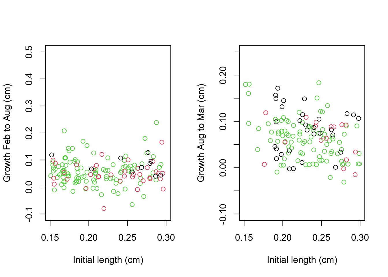
if(figs == "Y"){
  par(mfrow = c(1,2))
  plot(growth.1$Feb.Length, growth.1$growth.Aug.Feb, 
       col = as.factor(growth.1$Elevation),  
       ylim = c(-.1,.5), xlim = c(.15,.3),
       ylab = "Growth Feb to Aug (cm)",
       xlab = "Initial length (cm)"
  )
  plot(growth.2$Aug.Length, growth.2$growth.Mar.Aug, 
       col = as.factor(growth.2$Elevation), 
       ylim = c(-.1,.25), xlim = c(.15,.3), 
       ylab = "Growth Aug to Mar (cm)",
       xlab = "Initial length (cm)"
  )

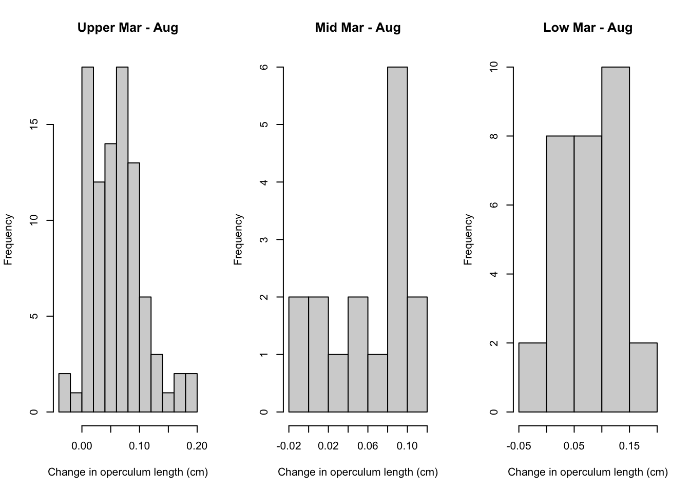
par(mfrow = c(1,3))
hist(growth.2$growth.Mar.Aug[growth.2$Elevation=="Upper"], 
     main = "Upper Mar - Aug", xlab = "Change in operculum length (cm)")
hist(growth.2$growth.Mar.Aug[growth.2$Elevation=="Mid"], 
     main = "Mid Mar - Aug", xlab = "Change in operculum length (cm)")
hist(growth.2$growth.Mar.Aug[growth.2$Elevation=="Low"], 
     main = "Low Mar - Aug", xlab = "Change in operculum length (cm)")
}

More growth plots and table

par(mfrow = c(1,2))

plot(as.factor(growth.2$Elevation), growth.2$growth.Mar.Aug, ylim = c(-.08, 0.25), ylab = "Growth (mm)", xlab = "Elevation")
plot(as.factor(growth.1$Elevation), growth.1$growth.Aug.Feb, ylim = c(-.08, 0.25), ylab = "", xlab = "Elevation")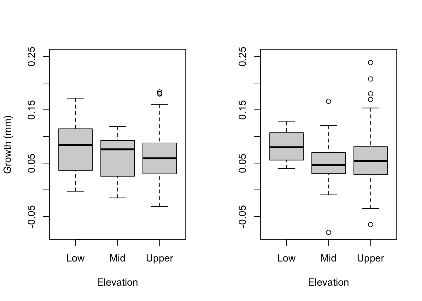

# No interactions:
par(mfrow = c(1,2))
# summary(lm(growth.1$growth.Aug.Feb~as.factor(growth.1$Elevation)+as.numeric(growth.1$Feb.Length)))

# Time 1
mod1 <- lm(growth.Aug.Feb~Elevation*Feb.Length, data = growth.1)
kbl(coef(summary(mod1)))%>%
  kable_classic_2(full_width = F)

	Estimate	Std. Error	t value	Pr(>\|t\|)
(Intercept)	0.1506457	0.0910366	1.6547820	0.1001023
ElevationMid	-0.1066055	0.0999380	-1.0667167	0.2878486
ElevationUpper	-0.0981680	0.0941666	-1.0424921	0.2988950
Feb.Length	-0.2727793	0.3539495	-0.7706730	0.4421377
ElevationMid:Feb.Length	0.2927743	0.3934002	0.7442148	0.4579346
ElevationUpper:Feb.Length	0.2992674	0.3718298	0.8048505	0.4222058

  # No interactions
mod1 <- lm(growth.Aug.Feb~Elevation+Feb.Length, data = growth.1)
kbl(coef(summary(mod1)))%>%
  kable_classic_2(full_width = F)

	Estimate	Std. Error	t value	Pr(>\|t\|)
(Intercept)	0.0802769	0.0275039	2.9187498	0.0040599
ElevationMid	-0.0325974	0.0168518	-1.9343539	0.0549646
ElevationUpper	-0.0232475	0.0160775	-1.4459641	0.1502874
Feb.Length	0.0045558	0.0912726	0.0499146	0.9602573

dat1.emm <- emmeans(mod1, "Elevation")
# plot(dat1.emm)
#emmeans::emmip(mod1, growth.Mar.Aug ~ Elevation , CIs = TRUE)
dat1.emm.df <- as.data.frame(dat1.emm)
mid <- barplot(data = dat1.emm.df, emmean~Elevation, 
               ylim = c(0,.15), ylab = "Size-corrected growth (cm per 6-months)")
arrows(x0=mid, y0=dat1.emm.df$lower.CL, x1=mid, 
       y1=dat1.emm.df$upper.CL, code = 3, angle=90, 
       length=0.1)
(0.08126638 - 0.05801888) / 0.05801888

[1] 0.4006885

# Time 2
mod1 <- lm(data = growth.2, growth.Mar.Aug~Elevation*Aug.Length)
kbl(coef(summary(mod1)))%>%
  kable_classic_2(full_width = F)

	Estimate	Std. Error	t value	Pr(>\|t\|)
(Intercept)	0.0927026	0.0558446	1.6600097	0.0992863
ElevationMid	0.0459385	0.0940378	0.4885109	0.6259986
ElevationUpper	0.0819102	0.0633740	1.2924890	0.1984458
Aug.Length	-0.0510427	0.2420486	-0.2108778	0.8333078
ElevationMid:Aug.Length	-0.2535982	0.3842576	-0.6599694	0.5104234
ElevationUpper:Aug.Length	-0.4437342	0.2742084	-1.6182370	0.1079986

  # No interactions
mod1 <- lm(data = growth.2, growth.Mar.Aug~Elevation+Aug.Length)
kbl(coef(summary(mod1)))%>%
  kable_classic_2(full_width = F)

	Estimate	Std. Error	t value	Pr(>\|t\|)
(Intercept)	0.1689942	0.0256045	6.6001825	0.0000000
ElevationMid	-0.0101646	0.0137095	-0.7414298	0.4597303
ElevationUpper	-0.0195878	0.0091685	-2.1364360	0.0344612
Aug.Length	-0.3851085	0.1065605	-3.6139895	0.0004255

dat1.emm <- emmeans(mod1, "Elevation")
# plot(dat1.emm)
#emmeans::emmip(mod1, growth.Mar.Aug ~ Elevation , CIs = TRUE)
dat1.emm.df <- as.data.frame(dat1.emm)
mid <- barplot(data = dat1.emm.df, emmean~Elevation, 
               ylim = c(0,.15), ylab = "")
arrows(x0=mid, y0=dat1.emm.df$lower.CL, x1=mid, 
       y1=dat1.emm.df$upper.CL, code = 3, angle=90, 
       length=0.1)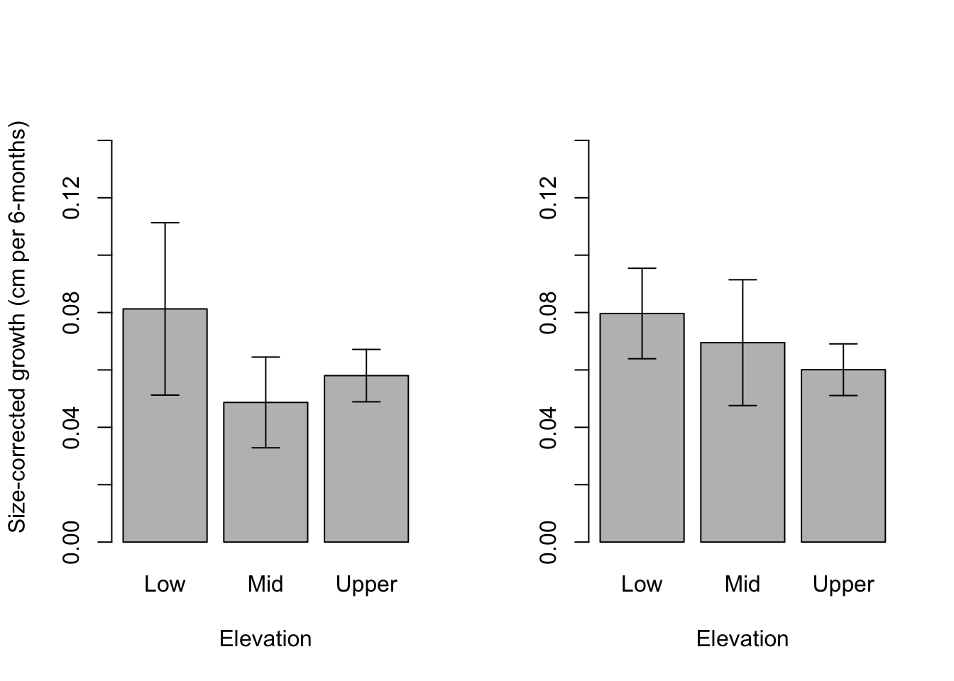

(0.08086259 - 0.05984264) / 0.05984264

[1] 0.3512537

Timepoint_1 <- as.POSIXct( "2018-02-04", format="%Y-%m-%d", tz = "GMT")
# Timepoint_2 <- as.POSIXct( "2018-08-13", format="%Y-%m-%d", tz = "GMT") #Changed 20210405 to avoid 1 day gap in data as loggers were switched out and photos were taken
Timepoint_1_end <- as.POSIXct( "2018-08-12", format="%Y-%m-%d", tz = "GMT")
Timepoint_2_start <- as.POSIXct( "2018-08-15", format="%Y-%m-%d", tz = "GMT")
Timepoint_3 <- as.POSIXct( "2019-03-01", format="%Y-%m-%d", tz = "GMT")

7 Relationship between operculum and tissue mass

This information is not used in this model. It was used for the previous analysis of the larger barnacles.

Larger barnacles did not change in opercular length much, but their tissue mass and condition index varied. We were not able to quantify reproductive ouput, and reproductive timing confounded tissue gain and loss of larger barnacles. Given this issue, we chose to focus on the growth rates of small barnacles.

# ============================#
# Read in tissue mass data ####
# ============================#
#setwd("C:/Users/eroberts/Box/Sarah and Molly's Box/FHL data/length mass relationship/FHL Collected Barnacles")
#setwd("~/Box/Sarah and Molly's Box/FHL data/length mass relationship/FHL Collected Barnacles")

setwd("~/Library/CloudStorage/Box-Box/Sarah and Molly's Box/FHL data/length mass relationship/FHL Collected Barnacles")
len_mass_Feb18 <- read.csv(file = "FHL 201803_Mar.csv", stringsAsFactors = FALSE)
len_mass_Aug18 <- read.csv(file = "FHL 201808_Aug.csv", stringsAsFactors = FALSE)
len_mass_Mar19 <- read.csv(file = "FHL 201903_Mar.csv", stringsAsFactors = FALSE)

8 Read in temperature data

Visually, this looks like: High – 1.97 m = 6.46 ft Mid – 1.55 m = 5.08 ft Low – 1.20 m = 3.93 ft Bars denote plus or minus 0.05 m (= 0.16 ft)

In email January 8, 2020, Gordon got: High = 1.98m Mid = 1.58m Low = 1.18m

From diagrams I know that the whole setup is about 3.5 ft from bottom to top, with 1 ft in between each layer of tiles. More like 2.5 bc not at edge

#setwd("~/Box/Sarah and Molly's Box/FHL data/HOBO data/Tides")
#setwd("C:/Users/eroberts/Box/Sarah and Molly's Box/FHL data/HOBO data/Tides")
# setwd("~/Library/CloudStorage/Box-Box/Sarah and Molly's Box/FHL data/HOBO data/Tides")
# setwd("~/Documents/GitHub/Bglandula_FHL_energetics/data/environmental_data")
# READING IN NEW TEMP DATASET ####
tempdat <- read.csv(here::here("data/environmental_data/TempAndWaterLevel_QC.20210401.csv"), stringsAsFactors = FALSE) #This is saved in r code HoboCombineFHL...v4.R
str(tempdat)

'data.frame':   54803 obs. of  7 variables:
 $ X          : int  1 2 3 4 5 6 7 8 9 10 ...
 $ datetime   : chr  "2017-08-07 00:45:00" "2017-08-07 01:00:00" "2017-08-07 01:15:00" "2017-08-07 01:30:00" ...
 $ Upper      : num  13.7 14.2 14.1 14.1 14 ...
 $ Mid        : num  13.3 14.2 14.1 14.1 14.1 ...
 $ Low        : num  13.2 14.1 14 14 14 ...
 $ Water.Level: num  NA 2.23 2.26 2.29 2.3 ...
 $ Water.Temp : num  16.1 12.8 11.6 11.8 12.8 ...

tempdat$datetime <- as.POSIXct(tempdat$datetime, tz = "GMT")
df.new <- tempdat
tempdat <- tempdat[!is.na(tempdat$Water.Level),]

subsetcheck1 <- as.POSIXct("2018-08-20 00:00:00")
subsetcheck2 <- as.POSIXct("2018-08-26 00:00:00")
tempdat_subset <- tempdat[tempdat$datetime > subsetcheck1&tempdat$datetime < subsetcheck2,]

tempdat$Upper_air <- tempdat$Upper
tempdat$Upper_water <- tempdat$Upper
tempdat$Upper_air[tempdat$Water.Level>=1.97] <- NA
tempdat$Upper_water[tempdat$Water.Level<1.97] <- NA

par(mfrow = c(1,3))
# plot(tempdat$Upper_air ~ tempdat$datetime, col = "red")
# points(tempdat$Upper_water ~ tempdat$datetime, col = "blue")
plot(tempdat$Upper_air ~ tempdat$datetime, col = "red")
points(tempdat$Upper_water ~ tempdat$datetime, col = "blue")

tempdat$Mid_air <- tempdat$Mid
tempdat$Mid_water <- tempdat$Mid
tempdat$Mid_air[tempdat$Water.Level>=1.55] <- NA
tempdat$Mid_water[tempdat$Water.Level<1.55] <- NA
plot(tempdat$Mid_air ~ tempdat$datetime, col = "red")
points(tempdat$Mid_water ~ tempdat$datetime, col = "blue")

tempdat$Low_air <- tempdat$Low
tempdat$Low_water <- tempdat$Low
tempdat$Low_air[tempdat$Water.Level>=1.20] <- NA
tempdat$Low_water[tempdat$Water.Level<1.20] <- NA
plot(tempdat$Low_air ~ tempdat$datetime, col = "red")
points(tempdat$Low_water ~ tempdat$datetime, col = "blue")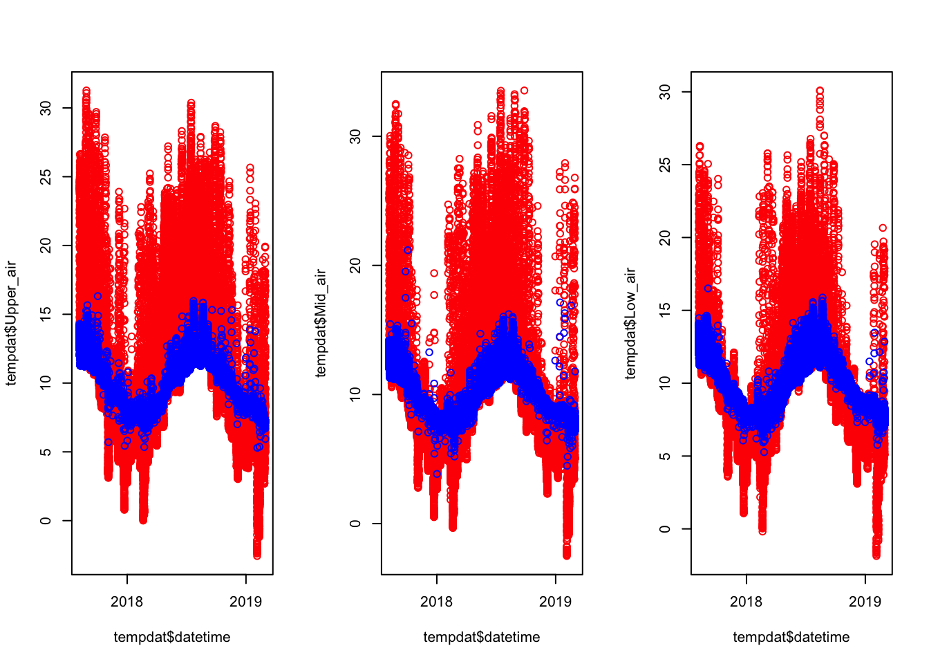

water.temp <- data.frame(
  datetime = tempdat$datetime,
  Upper = tempdat$Upper_water,
  Mid = tempdat$Mid_water,
  Low = tempdat$Low_water)

air.temp <- data.frame(
  datetime = tempdat$datetime,
  Upper = tempdat$Upper_air,
  Mid = tempdat$Mid_air,
  Low = tempdat$Low_air)



#if(timing == 1){ 
  starttime <- Timepoint_1
  endtime <- Timepoint_1_end
  air.temp.1 <- air.temp[air.temp$datetime>=starttime & air.temp$datetime<= endtime & !is.na(air.temp$datetime),]
  water.temp.1 <- water.temp[water.temp$datetime>=starttime & water.temp$datetime<= endtime & !is.na(water.temp$datetime),]
#}

#if(timing == 2){
  starttime <- Timepoint_2_start
  endtime <- Timepoint_3
  air.temp.2 <- air.temp[air.temp$datetime>=starttime & air.temp$datetime<= endtime & !is.na(air.temp$datetime),]
  water.temp.2 <- water.temp[water.temp$datetime>=starttime & water.temp$datetime<= endtime & !is.na(water.temp$datetime),]
#}
  
  
  par(mfrow = c(1,1))

plot(tempdat$Upper, pch = ".")
points(tempdat$Mid, col = "blue", pch=".")
points(tempdat$Low, col = "orange", pch = ".")
title("Temps at the 3 tidal elevations over 1 year")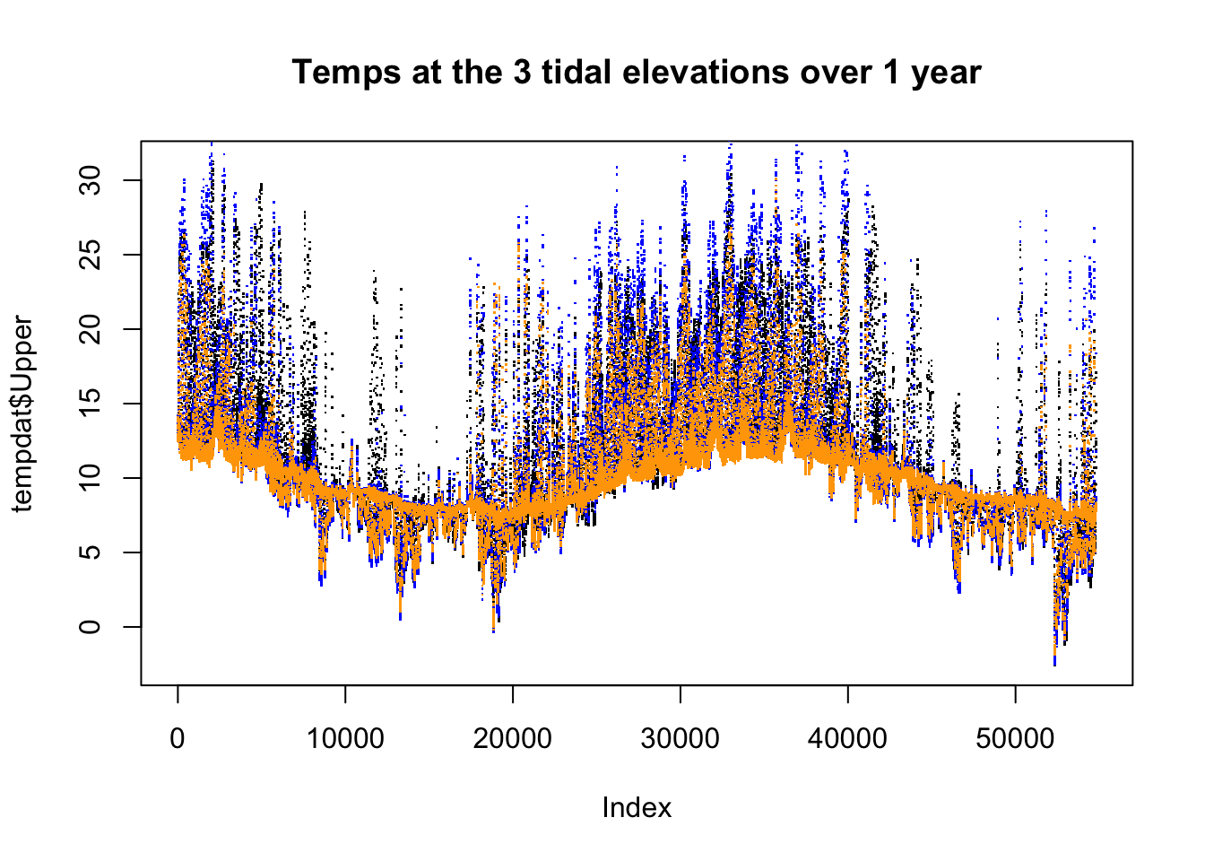

plot(tempdat_subset$Upper, pch = ".")
points(tempdat_subset$Mid, col = "blue", pch=".")
points(tempdat_subset$Low, col = "orange", pch = ".")
title("Temps of the 3 tidal elevations over one week")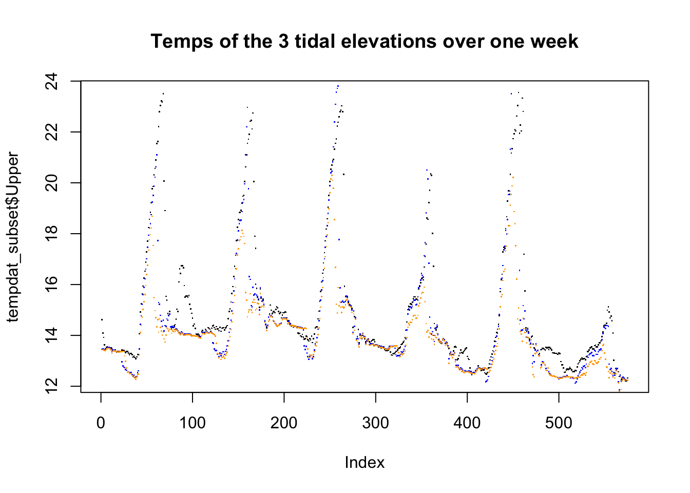

plot(air.temp.1$Upper, pch = ".")
points(air.temp.1$Mid, col = "blue", pch=".")
points(air.temp.1$Low, col = "orange", pch = ".")
title("Temps of the 3 tidal elevations over the first 6-month experiment")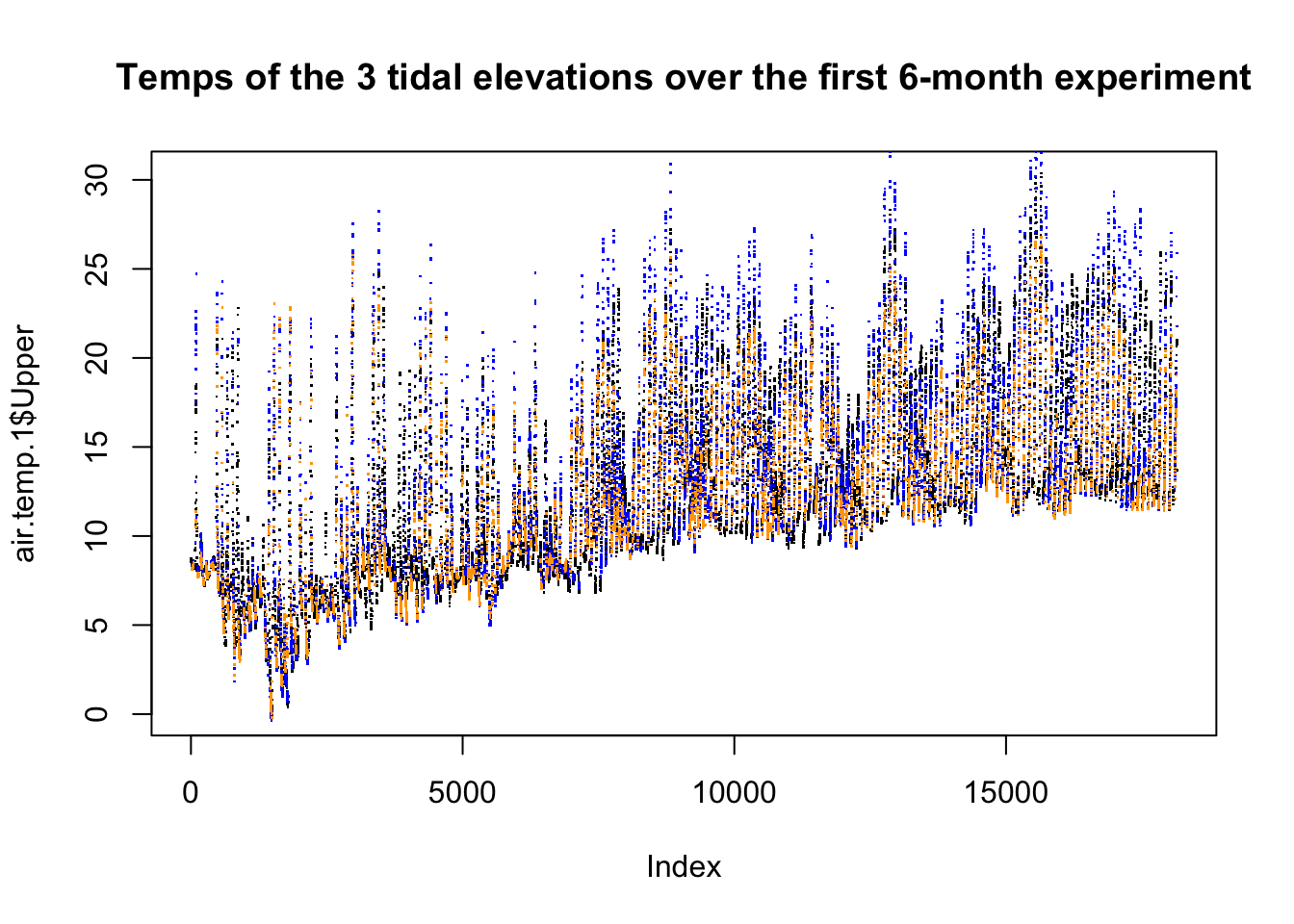

plot(air.temp.2$Upper, pch = ".")
points(air.temp.2$Mid, col = "blue", pch=".")
points(air.temp.2$Low, col = "orange", pch = ".")
title("Temps of the 3 tidal elevations over the second 6-month experiment")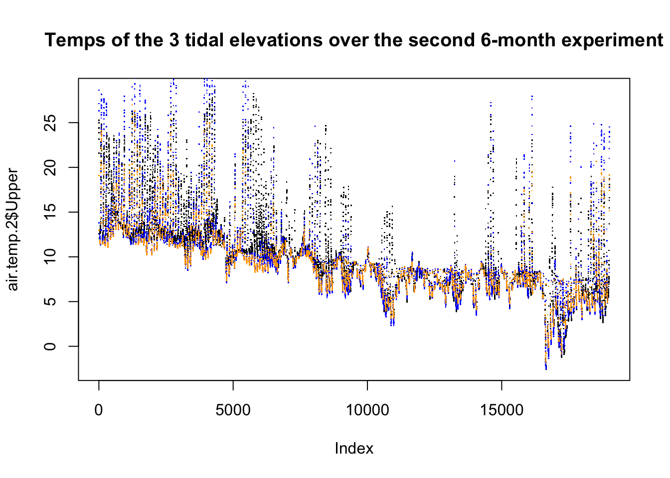

9 Food data

Data found in:

#setwd(“~/Box/Sarah and Molly’s Box/FHL data/SONDE data/Padilla Bay/909184_all_data_2003topresent”)

setwd(“C:/Users/eroberts/Box/Sarah and Molly’s Box/FHL data/SONDE data/Padilla Bay/909184_all_data_2003topresent”)

setwd(“~/Library/CloudStorage/Box-Box/Sarah and Molly’s Box/FHL data/SONDE data/Padilla Bay/909184_all_data_2003topresent/”)

Read in data

PB <- read.csv(here::here("data/environmental_data/PDBGSWQ_dataonly.csv"), stringsAsFactors = FALSE)

#Technically this should be in pdt, but this is being used to calculate weekly averages and lubridate is not working correctly
PB$datetime <-as.POSIXct(PB$m.d.y.hh.mm, format = "%m/%d/%y %H:%M", tz = "UTC")

#subset to only include the past 3 years...
time_zone <- "UTC"
PB_subset <- PB[PB$datetime > as.POSIXct("2017-01-01 00:00:00", tz = "UTC") & PB$datetime< as.POSIXct("2020-01-01 00:00:00", tz = time_zone),]
PB <- PB_subset

plot(PB$datetime, PB$ug.l, pch = ".")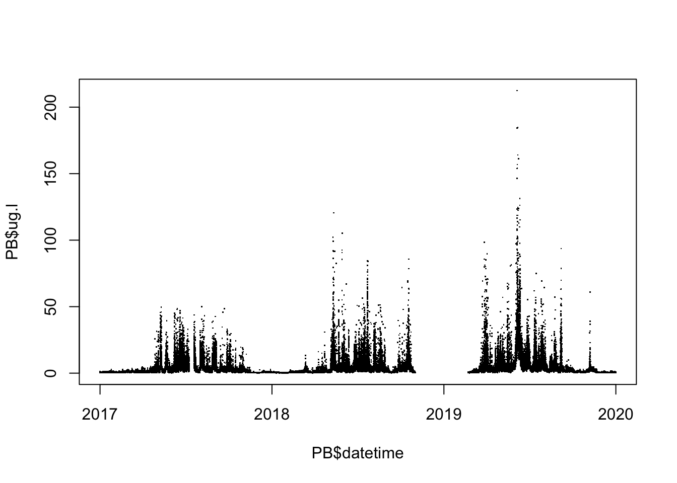

# plot(PB$datetime, PB$psu, pch = ".")

vars <-"m.d.y.hh.mm"
dat <- PB %>% 
  drop_na(ug.l, any_of(vars))%>%
  dplyr::group_by(time = week(datetime)) %>% 
  dplyr::summarise(value = mean(ug.l, na.rm = TRUE), .groups = 'keep')
dat

# A tibble: 53 × 2
# Groups:   time [53]
    time value
   <dbl> <dbl>
 1     1 0.632
 2     2 0.632
 3     3 0.611
 4     4 0.577
 5     5 0.486
 6     6 0.731
 7     7 0.869
 8     8 0.927
 9     9 1.11 
10    10 1.31 
# … with 43 more rows

plot(dat, type = 'b', ylab = "fluorescence (ug/L)", xlab = "week")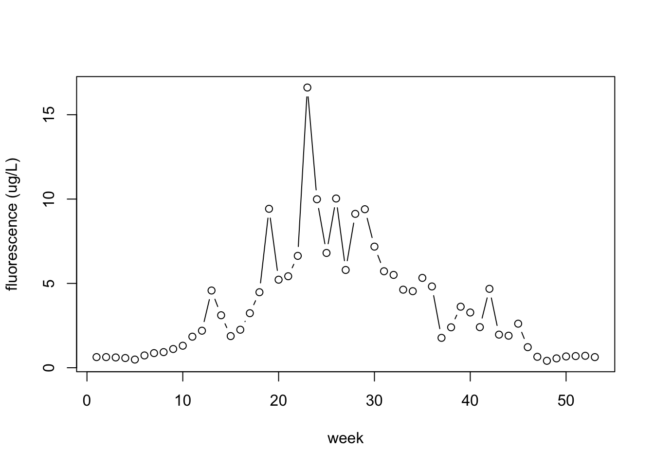

#dat$datetime.2017 <- lubridate::ymd_hms( "2017-01-01 00:00:01" ) + lubridate::weeks( dat$time - 1 )
dat$datetime.2018 <- lubridate::ymd_hms( "2018-01-01 00:00:01" ) + lubridate::weeks( dat$time - 1 )
dat$datetime.2019 <- lubridate::ymd_hms( "2019-01-01 00:00:01" ) + lubridate::weeks( dat$time - 1 )

food <- data.frame(
  datetime = as.POSIXct(c(dat$datetime.2018, dat$datetime.2019)),
  food = c(dat$value,dat$value)
)

plot(food)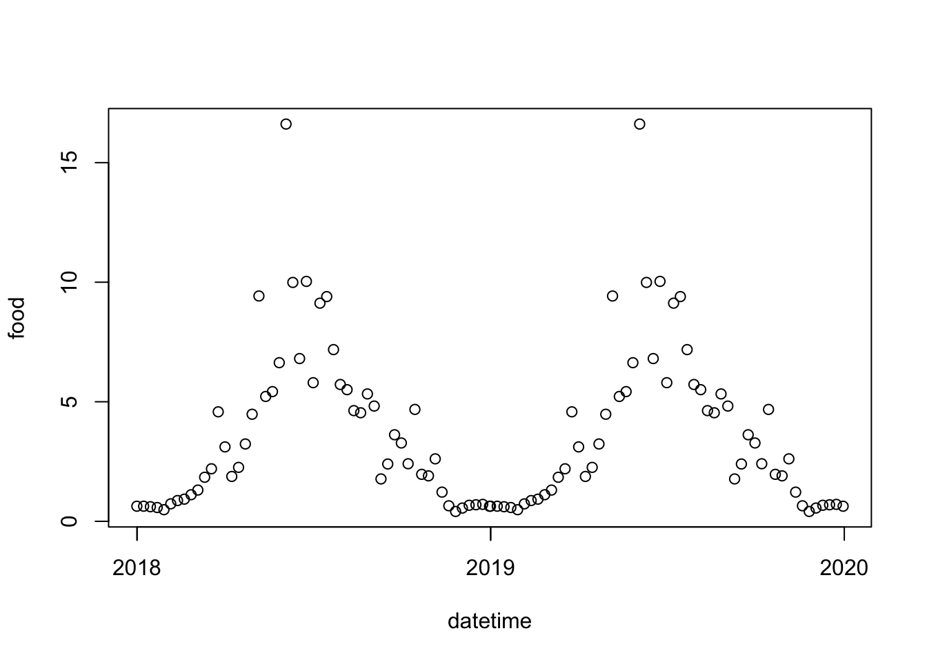

require(zoo)
# Create zoo library objects
zf <- zoo(food$food, food$datetime)   # low freq
zt <- zoo(water.temp.1$Upper, water.temp.1$datetime)  # high freq
z <- merge(zf,zt,all = TRUE)
z$zf <- na.approx(z$zf, rule=2)
food.interp <- fortify.zoo(z$zf)
names(food.interp) <- c("datetime", "food")
water.temp.1 <- left_join(water.temp.1, food.interp, by = "datetime")

zf <- zoo(food$food, food$datetime)   # low freq
zt <- zoo(water.temp.2$Upper, water.temp.2$datetime)  # high freq
z <- merge(zf,zt,all = TRUE)
z$zf <- na.approx(z$zf, rule=2)
food.interp <- fortify.zoo(z$zf)
names(food.interp) <- c("datetime", "food")
water.temp.2 <- left_join(water.temp.2, food.interp, by = "datetime")

Plots of chlorophyll

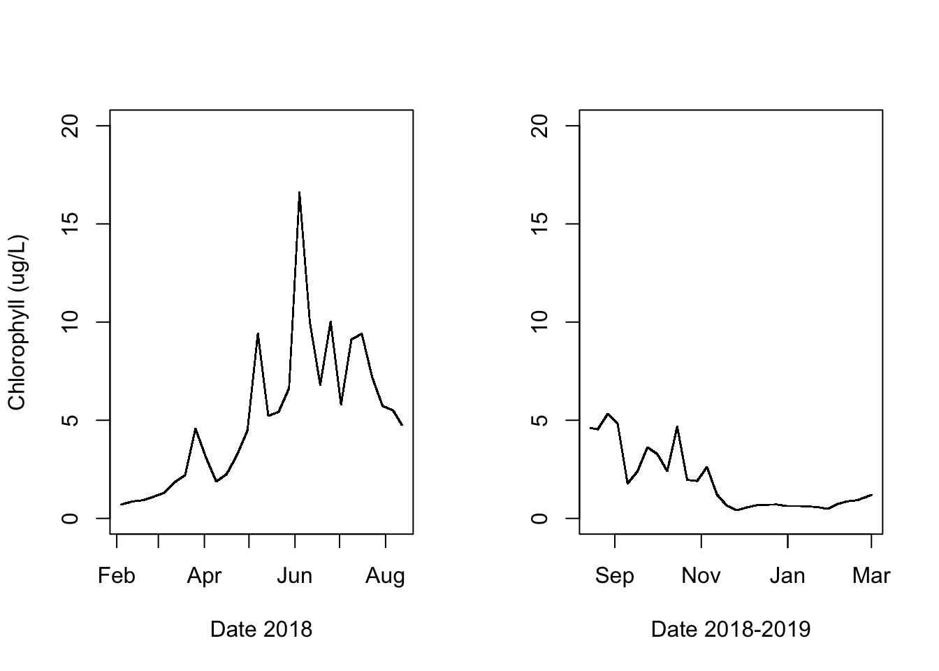
if(figs == "Y"){
par(mfrow = c(1,2))
plot(water.temp.1$food~ water.temp.1$datetime,
     ylim = c(0,20),
     ylab = "Chlorophyll (ug/L)",
     xlab = "Date 2018",
     pch = ".")
plot(water.temp.2$food~ water.temp.2$datetime,
     ylim = c(0,20),
     ylab = "",
     xlab = "Date 2018-2019",
     pch = ".")
}

Iter.len.1 <- as.data.frame(matrix(data = 0, ncol = nrow(growth.1), nrow = length(water.temp.1$datetime)))
Iter.len.1[1,] <- growth.1$Feb.Length

Iter.len.2 <- as.data.frame(matrix(data = 0, ncol = nrow(growth.2), nrow = length(water.temp.2$datetime)))
Iter.len.2[1,] <- growth.2$Aug.Length

10 Physiology: Thermal performance relationships

Read in feeding, respiration relationships

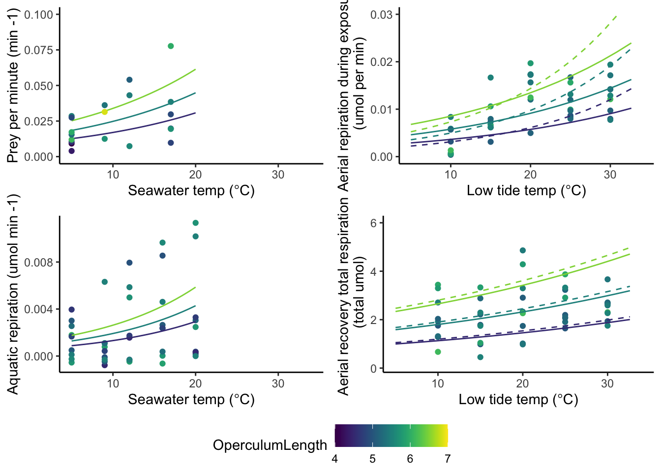
Feeding ~ Temp, Aquatic Respiration ~ Temp, Aerial Respiration ~ Temp Feeding shrimp per min ~ Temp C, Upslope to 20 degrees

Use a subset of the data, up to 20 degrees to interpolate feeding rate upslope,

Wu and Levings equation with random component, assuming allometric scaling factor

10.0.1 Feeding rate

Feeding shrimp per min ~ Temp C, Upslope to 20 degrees

Using the operculum length allometric factor of 1.88.

Data pulled from here:

#setwd(“~/Box/Sarah and Molly’s Box/FHL data/aqua feeding and resp”) # setwd(“C:/Users/eroberts/Box/Sarah and Molly’s Box/FHL data/aqua feeding and resp”) setwd(“~/Documents/GitHub/Bglandula_FHL_energetics/data/physiology_data”)

#old version of datafile
#feed<- read.table("aqfeedFHL.csv", header = T, sep = ",")

feed<- read.table(here::here("data/physiology_data/aqfeedFHL_log.csv"), header = T, sep = ",")
feed$Temp <- as.factor(feed$Temp)
feed$Temp.n <- as.numeric(as.character(feed$Temp))
feed_subset <- feed[feed$Temp.n <= 17,]
feed <- feed_subset
feed$feedrate.new <- feed$m_filter_300 - feed$a_ave
feed$feedrate <- feed$feedrate.new
feed <- feed[!is.na(feed$feedrate.new),]
feed$ID <- as.factor(feed$ID)
feed$bin <- bin(feed$OperculumLength, nbins = 3) #(4.02,4.97] (4.97,5.91] (5.91,6.86]
feed$sizeclass <- bin(feed$OperculumLength, nbins = 3, labels = c("small", "medium", "large"))

FR_T <- nls(feedrate ~ exp(a*Temp.n) * OperculumLength^(1.88) * c,
            data = feed, start = c(a = .1, c = .0004))
summary(FR_T)


Formula: feedrate ~ exp(a * Temp.n) * OperculumLength^(1.88) * c

Parameters:
   Estimate Std. Error t value Pr(>|t|)  
a 0.0593597  0.0285303   2.081   0.0520 .
c 0.0005550  0.0002197   2.527   0.0211 *
---
Signif. codes:  0 '***' 0.001 '**' 0.01 '*' 0.05 '.' 0.1 ' ' 1

Residual standard error: 0.0158 on 18 degrees of freedom

Number of iterations to convergence: 4 
Achieved convergence tolerance: 4.217e-06

FR_T_a <- coef(FR_T)[1]
FR_T_c <- coef(FR_T)[2]

FR_T_fun <- function(temp, size, a = FR_T_a, c = FR_T_c) {
  out <- exp(a * temp) * size^(1.88) * c
  return(out)
}

# Previous version:
# FR_T <- nlme(feedrate ~ exp(a * Temp.n) * OperculumLength^(1.86) * c,
#              data = feed,
#              fixed = a + c~ 1,
#              random = c ~ 1,
#              groups = ~ ID,
#              start = c(a = -.007, c = 100))
# summary(FR_T)
# FR_T_a <- FR_T$coefficients$fixed[[1]]
# FR_T_c <- FR_T$coefficients$fixed[[2]]

# FR_T_fun <- function(temp, size, a = FR_T_a, c = FR_T_c) {
#   out <- exp(a * temp) * size^(1.86) * c
#   return(out)
# }

pred.dat.aqua$feedrate <- FR_T_fun(pred.dat.aqua$Temp.n, pred.dat.aqua$OperculumLength)
pred.dat$feedrate <- FR_T_fun(temp = pred.dat$Temp.n, size = pred.dat$OperculumLength)

 gg1 <- ggplot(data = pred.dat.aqua, 
       aes(x = as.numeric(Temp.n), 
           y=as.numeric(feedrate), 
           color = OperculumLength, group = as.factor(sizeclass)))+
  geom_line()+
  scale_color_viridis(option = "D", limits = c(4, 7))+
  geom_point(data = feed,aes(x=Temp.n,y=feedrate,color=OperculumLength))+
  xlim(5,34)+
  ylim(0,.1)+
  xlab(expression(paste("Seawater temp (",degree,"C)")))+
  ylab("Prey per minute (min -1)")
gg1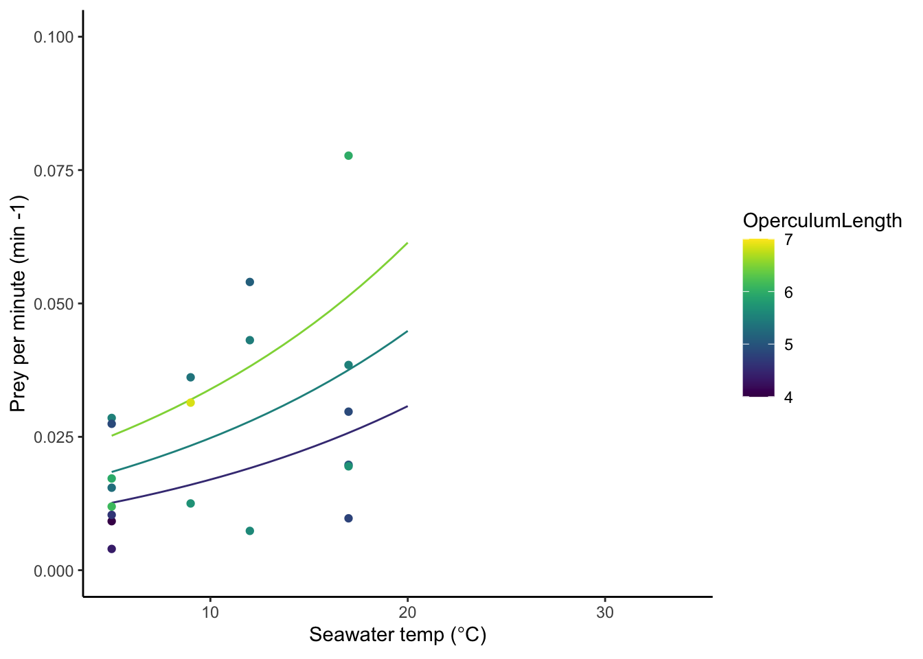

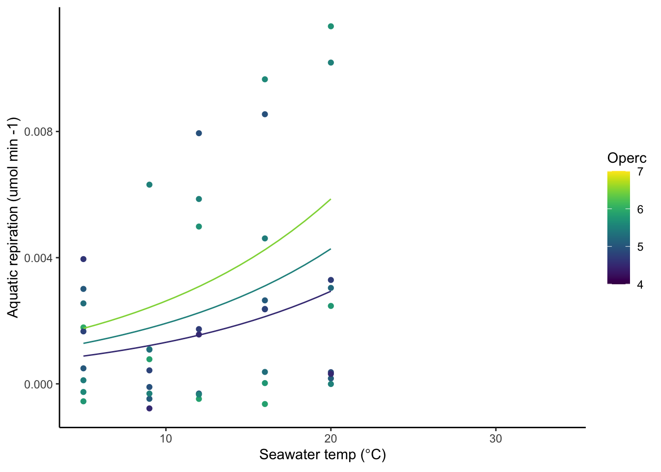
10.1 Aquatic respiration (umol oxygen per min) ~ Temp (deg C)

Upslope to 23 degrees

Use a subset of the data, up to 23 degrees to interpolate respiration rate upslope,

Wu and Levings equation with random component, assuming allometric scaling factor

Previously found:

setwd(“~/Box/Sarah and Molly’s Box/FHL data/aqua feeding and resp”) setwd(“C:/Users/eroberts/Box/Sarah and Molly’s Box/FHL data/aqua feeding and resp”)

resp<- read.table(here::here("data/physiology_data/AQtotalresp_FHL.csv"), header = T, sep = ",")
resp$Temp<- as.factor(resp$Temp)
resp$Operc

 [1] 5.11 5.11 5.11 5.99 5.99 5.99 5.03 5.03 5.03 5.75 5.75 5.75 5.22 5.22 4.87
[16] 4.87 4.87 5.86 5.86 5.86 4.63 4.63 4.63 5.77 5.77 5.77 5.46 5.46 5.46 4.50
[31] 4.50 4.50 5.07 5.07 5.07 5.70 5.70 5.70 4.95 4.95 4.95 5.29 5.29 5.29 4.80
[46] 4.80 4.80 5.05 5.05 5.05 4.70 4.70 4.70 5.51 5.51 5.51 5.51 5.51 5.51 5.60
[61] 5.60 5.60

resp$ID <- as.factor(resp$Barnacle)
resp$Temp.n <- as.numeric(as.character(resp$Temp))
resp$sizeclass <- bin(resp$Operc, nbins = 3, labels = c("small", "medium", "large"))
resp$bin <- bin(resp$Operc, nbins = 3) #(4.02,4.97] (4.97,5.91] (5.91,6.86]

resp_below_23 <- resp[resp$Temp.n < 23,] #Changed 2020 Aug 12
resp <- resp_below_23

AQR_T <- nlme(Respiration.Rate ~ c * exp(a * Temp.n) * Operc^1.88,
              data = resp,
              fixed = a + c ~ 1,
              random = c ~ 1,
              groups = ~ ID,
              start = c(a = 0.0547657, c = 0.0003792))
summary(AQR_T)

Nonlinear mixed-effects model fit by maximum likelihood
  Model: Respiration.Rate ~ c * exp(a * Temp.n) * Operc^1.88 
  Data: resp 
        AIC       BIC   logLik
  -379.3246 -372.1878 193.6623

Random effects:
 Formula: c ~ 1 | ID
                   c    Residual
StdDev: 9.908437e-09 0.002966555

Fixed effects:  a + c ~ 1 
       Value  Std.Error DF  t-value p-value
a 0.08030545 0.04076867 22 1.969783  0.0616
c 0.00003485 0.00002405 22 1.448871  0.1615
 Correlation: 
  a     
c -0.966

Standardized Within-Group Residuals:
       Min         Q1        Med         Q3        Max 
-1.4500246 -0.7135749 -0.2393238  0.4736441  2.2773886 

Number of Observations: 44
Number of Groups: 21

AQR_T_a <- AQR_T$coefficients$fixed[[1]]
AQR_T_c <- AQR_T$coefficients$fixed[[2]]

AQR_T_fun <- function(temp, size, c = AQR_T_c, a = AQR_T_a) {
  out <- c * exp(a * temp) * size^1.88
  return(out)
}


pred.dat.aqua$aq_resp <- AQR_T_fun(temp = pred.dat.aqua$Temp.n, size = pred.dat.aqua$OperculumLength)
pred.dat$aq_resp <- AQR_T_fun(temp = pred.dat$Temp.n, size = pred.dat$OperculumLength)

if(figs == "Y"){

    # ggplot(resp,aes(x=Temp.n,y=Respiration.Rate,color=factor(sizeclass)))+
    #   geom_point()+
    #   geom_line(data = pred.dat.aqua, 
    #             aes(x = as.numeric(Temp.n), 
    #                 y=as.numeric(aq_resp), 
    #                 color = factor(sizeclass)))+
    #   xlim(5,18)+
    #   ylim(0,.01)

resp_aq <- resp
gg2 <- ggplot(resp_aq,aes(x=Temp.n,y=Respiration.Rate,color=Operc))+
    geom_point()+
    scale_color_viridis(option = "D", limits = c(4,7))+
    geom_line(data = pred.dat.aqua, 
              aes(x = as.numeric(Temp.n), 
                  y=as.numeric(aq_resp), 
                  color = OperculumLength, group = as.factor(sizeclass)))+
    xlim(5,34)+
    # ylim(0,.01)+
    xlab(expression(paste("Seawater temp (",degree,"C)")))+
    ylab("Aquatic repiration (umol min -1)")
gg2  

    }

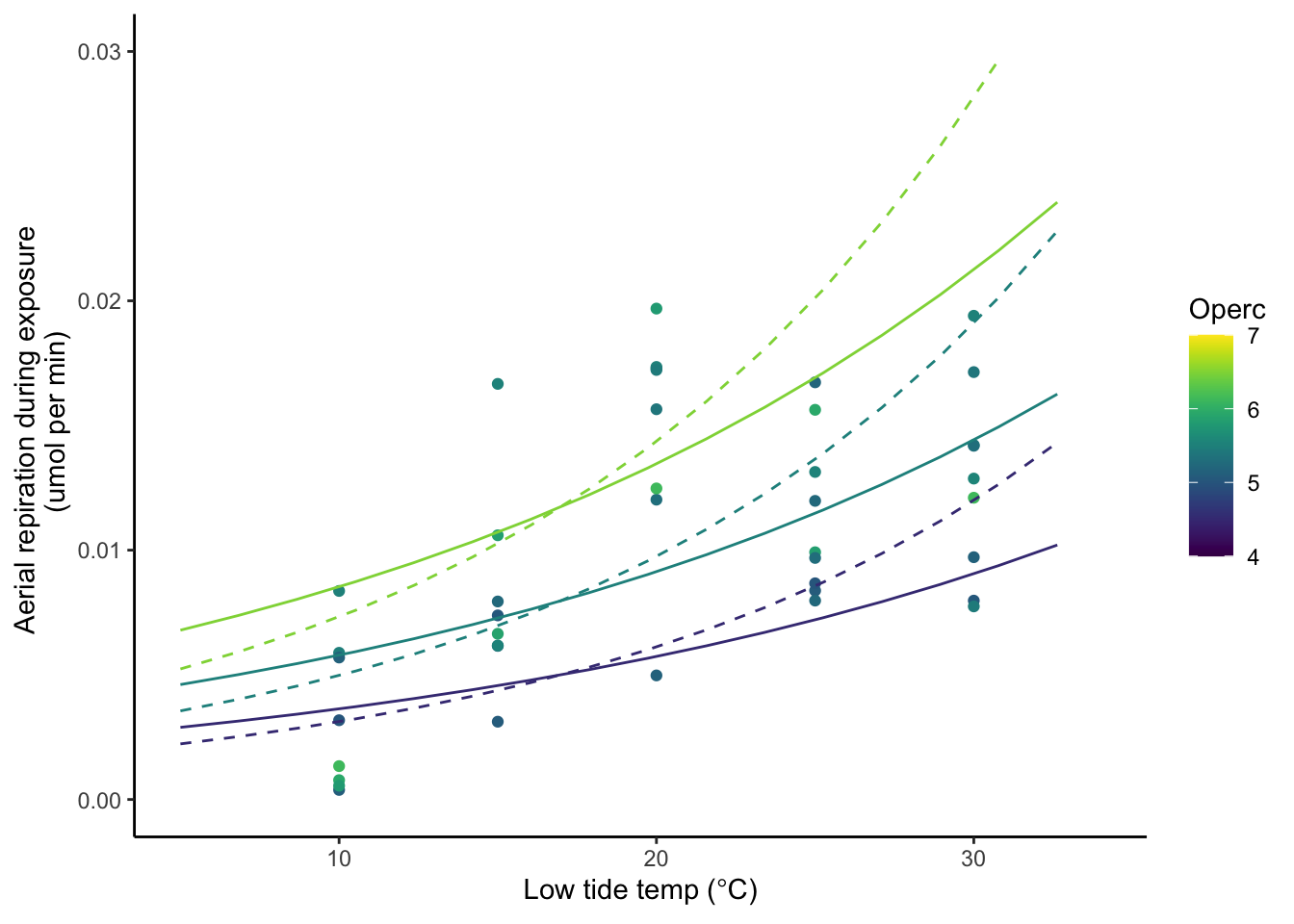
10.2 Aerial exposure respiration (umol oxygen per 15 min) ~ Temp (deg C)

Upslope to 25 deg, 30 deg, and quadratic

Two hypotheses: Upslope vs. unimodal hypothesis

Data originally here:

setwd(“~/Box/Sarah and Molly’s Box/FHL data/aerial resp”) setwd(“C:/Users/eroberts/Box/Sarah and Molly’s Box/FHL data/aerial resp”)

resp<- read.csv(here::here("data/physiology_data/FHLmean15mins_recovery_forMolly_40deg.csv"), stringsAsFactors = FALSE, header = T, sep = ",")
resp$Temp<- as.factor(resp$Temp)
resp$Operc <- resp$operculum_length
resp$Temp.n <- as.numeric(as.character(resp$Temp))
resp$Respiration.Rate <- resp$air_15min
resp$Barnacle <- as.factor(resp$Barnacle)
resp$sizeclass <- bin(resp$Operc, nbins = 3, labels = c("small", "medium", "large"))
resp$bin <- bin(resp$Operc, nbins = 3) #(4.02,4.97] (4.97,5.91] (5.91,6.86]

resp_below_30 <- resp[resp$Temp.n <= 30,]
resp_below_25 <- resp[resp$Temp.n <= 25,]

AER_EXPOSE_T_25 <- nlme(Respiration.Rate ~ c * exp(a * Temp.n) * Operc^2.32,
                        data = resp_below_25,
                        fixed = a + c ~ 1,
                        random = c ~ 1,
                        groups = ~ Barnacle,
                        start = c(a = 0.0547657, c = 0.0003792))
summary(AER_EXPOSE_T_25)

Nonlinear mixed-effects model fit by maximum likelihood
  Model: Respiration.Rate ~ c * exp(a * Temp.n) * Operc^2.32 
  Data: resp_below_25 
        AIC      BIC   logLik
  -79.53297 -73.1989 43.76649

Random effects:
 Formula: c ~ 1 | Barnacle
                   c   Residual
StdDev: 2.586767e-08 0.07174233

Fixed effects:  a + c ~ 1 
       Value   Std.Error DF  t-value p-value
a 0.06727408 0.018785384 14 3.581193  0.0030
c 0.00072931 0.000296084 14 2.463202  0.0273
 Correlation: 
  a     
c -0.976

Standardized Within-Group Residuals:
       Min         Q1        Med         Q3        Max 
-2.0695968 -0.7307817 -0.1549091  0.5659112  2.0172261 

Number of Observations: 36
Number of Groups: 21

AER_EXPOSE_T_25_a <- AER_EXPOSE_T_25$coefficients$fixed[[1]]
AER_EXPOSE_T_25_c <- AER_EXPOSE_T_25$coefficients$fixed[[2]]

AER_EXPOSE_T_30 <- nlme(Respiration.Rate ~ c * exp(a * Temp.n) * Operc^2.32,
                        data = resp_below_30,
                        fixed = a + c ~ 1,
                        random = c ~ 1,
                        groups = ~ Barnacle,
                        start = c(a = 0.0547657, c = 0.0003792))
summary(AER_EXPOSE_T_30)

Nonlinear mixed-effects model fit by maximum likelihood
  Model: Respiration.Rate ~ c * exp(a * Temp.n) * Operc^2.32 
  Data: resp_below_30 
        AIC       BIC   logLik
  -101.7062 -94.47956 54.85311

Random effects:
 Formula: c ~ 1 | Barnacle
                  c   Residual
StdDev: 4.49608e-08 0.07151154

Fixed effects:  a + c ~ 1 
       Value   Std.Error DF  t-value p-value
a 0.04562355 0.011564376 23 3.945181  0.0006
c 0.00105427 0.000304119 23 3.466623  0.0021
 Correlation: 
  a     
c -0.967

Standardized Within-Group Residuals:
        Min          Q1         Med          Q3         Max 
-1.96859864 -0.61433908 -0.05521089  0.46918810  1.96195111 

Number of Observations: 45
Number of Groups: 21

AER_EXPOSE_T_30_a <- AER_EXPOSE_T_30$coefficients$fixed[[1]]
AER_EXPOSE_T_30_c <- AER_EXPOSE_T_30$coefficients$fixed[[2]]

AER_EXPOSE_T_all <- nlme(Respiration.Rate ~ c * exp(a1*Temp.n) * exp(a2*Temp.n^2) * Operc^2.32,
                         data = resp,
                         fixed = a1 + a2 + c ~ 1,
                         random = c ~ 1,
                         groups = ~ Barnacle,
                         start = c(a1 = 2.201e-01, a2 = -4.623e-03, c = 1.433e-05))
summary(AER_EXPOSE_T_all)

Nonlinear mixed-effects model fit by maximum likelihood
  Model: Respiration.Rate ~ c * exp(a1 * Temp.n) * exp(a2 * Temp.n^2) *      Operc^2.32 
  Data: resp 
        AIC      BIC   logLik
  -134.7807 -124.065 72.39035

Random effects:
 Formula: c ~ 1 | Barnacle
                   c   Residual
StdDev: 1.911226e-09 0.07668941

Fixed effects:  a1 + a2 + c ~ 1 
         Value  Std.Error DF   t-value p-value
a1  0.19135365 0.05626881 40  3.400706  0.0015
a2 -0.00335510 0.00105077 40 -3.192979  0.0027
c   0.00025335 0.00018253 40  1.388047  0.1728
 Correlation: 
   a1     a2    
a2 -0.988       
c  -0.979  0.938

Standardized Within-Group Residuals:
       Min         Q1        Med         Q3        Max 
-2.0738357 -0.7486660 -0.2012656  0.4367642  3.4985767 

Number of Observations: 63
Number of Groups: 21

AER_EXPOSE_T_all_a1 <- AER_EXPOSE_T_all$coefficients$fixed[[1]]
AER_EXPOSE_T_all_a2 <- AER_EXPOSE_T_all$coefficients$fixed[[2]]
AER_EXPOSE_T_all_c <- AER_EXPOSE_T_all$coefficients$fixed[[3]]

Set functions

# Aerial exposure respiration rate
AER_EXPOSE_T_25_fcn <- function(temp, size, c = AER_EXPOSE_T_25_c, a = AER_EXPOSE_T_25_a) {
  out <- c * exp(a * temp) * size^2.32
  return(out)
}
AER_EXPOSE_T_30_fcn <- function(temp, size, c = AER_EXPOSE_T_30_c, a = AER_EXPOSE_T_30_a) {
  out <- c * exp(a * temp) * size^2.32
  return(out)
}
AER_EXPOSE_T_all_fcn <- function(temp, size, c = AER_EXPOSE_T_all_c, a1 = AER_EXPOSE_T_all_a1, a2 = AER_EXPOSE_T_all_a2) {
  out <- c * exp(a1 * temp) * exp(a2 * temp^2) * size^2.32
  return(out)
}

10.2.0.1 Compare predicted respiration curves from aerial exposure.

The dashed line indicates the growth curve when data up to 25C is used.

The solid line indicates the growth curve when data up to 30C is used.

# predicted values of respiration at a particular size and temp, above and below the graph axis limits won't be included on the graph, and this will produce an unnecessary warning

# Predicted values based on temp and size and function
pred.dat$pred_25 <- AER_EXPOSE_T_25_fcn(pred.dat$Temp.n, pred.dat$Operc)
pred.dat$pred_30 <- AER_EXPOSE_T_30_fcn(pred.dat$Temp.n, pred.dat$Operc)
pred.dat$pred_all <- AER_EXPOSE_T_all_fcn(pred.dat$Temp.n, pred.dat$Operc)
pred.dat.air$pred_25 <- AER_EXPOSE_T_25_fcn(pred.dat.air$Temp.n, pred.dat.air$Operc)
pred.dat.air$pred_30 <- AER_EXPOSE_T_30_fcn(pred.dat.air$Temp.n, pred.dat.air$Operc)
pred.dat.air$pred_all <- AER_EXPOSE_T_all_fcn(pred.dat.air$Temp.n, pred.dat.air$Operc)
pred.dat.air$air_resp_exposure_25 <- AER_EXPOSE_T_25_fcn(temp = pred.dat.air$Temp.n, size = pred.dat.air$OperculumLength)
pred.dat.air$air_resp_exposure_30 <- AER_EXPOSE_T_30_fcn(temp = pred.dat.air$Temp.n, size = pred.dat.air$OperculumLength)
pred.dat.air$air_resp_exposure_all <- AER_EXPOSE_T_all_fcn(temp = pred.dat.air$Temp.n, size = pred.dat.air$OperculumLength)


if(figs == "Y"){
  # ggplot(resp,aes(x=Temp.n,y=Respiration.Rate,color=factor(sizeclass)))+
  #   geom_point()+
  #   ylab("Aerial Respiration (umol per 15 min)") +
  #   xlab("Temp (deg C)")+
  #   geom_line(data = pred.dat, aes(x = as.numeric(Temp.n),
  #                                  y=as.numeric(pred_30), color = factor(sizeclass)), linetype = "dashed")+
  #   geom_line(data = pred.dat, aes(x = as.numeric(Temp.n),
  #                                  y=as.numeric(pred_all), color = factor(sizeclass)), linetype = "dotted")+
  #   geom_line(data = pred.dat, aes(x = as.numeric(Temp.n),
  #                                  y=as.numeric(pred_25), color = factor(sizeclass)), linetype = "solid")
  resp_exp <- resp
  gg3 <- ggplot(resp_exp,aes(x=Temp.n,y=Respiration.Rate/15,color=Operc))+
    geom_point()+
    scale_color_viridis(option = "D", limits = c(4,7))+
    geom_line(data = pred.dat.air, 
              aes(x = as.numeric(Temp.n), 
                  y=as.numeric(pred_25)/15, 
                  color = OperculumLength, group = as.factor(sizeclass)), linetype = "dashed")+
    geom_line(data = pred.dat.air, 
              aes(x = as.numeric(Temp.n), 
                  y=as.numeric(pred_30)/15, 
                  color = OperculumLength, group = as.factor(sizeclass)))+
    xlim(5,34)+
    ylim(0,.03)+
    xlab(expression(paste("Low tide temp (",degree,"C)")))+
    ylab("Aerial repiration during exposure \n (umol per min)")
  gg3  
  }

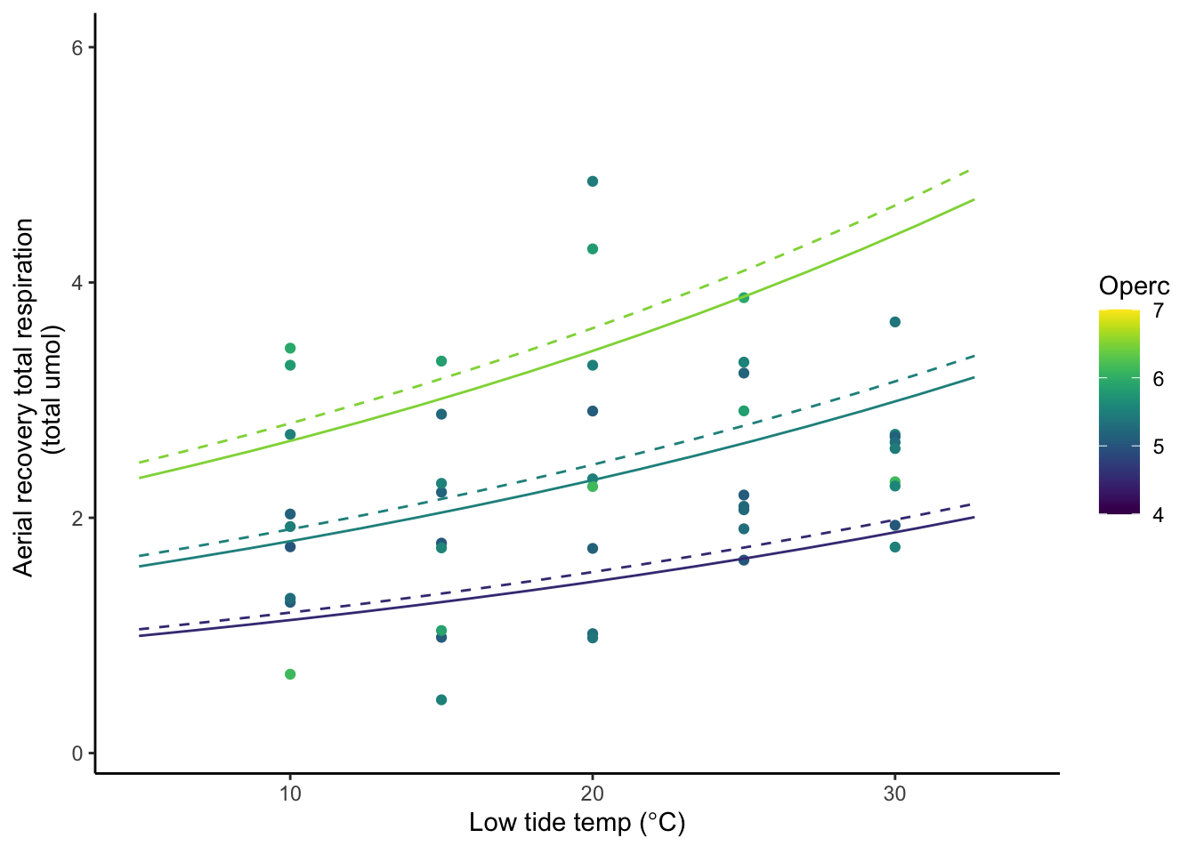
10.3 Aerial recovery respiration ~ Temp

We start with umol oxygen total, but then calculate umol oxygen per 15 min exposure # Upslope to 30 deg C